By: Jay Turcot, Lead Scientist

As we mentioned in Part 1 of our blog, our machine learning system consists of two primary components: data and algorithms. Machines, like students, learn through observing patterns and trends in many real life examples.

To make an analogy with a classroom setting: the algorithms are the students, the data are the teaching materials from which they learn. In this blog we will explore the algorithms and how these use the data in order to recognize emotions. To learn more about what role “data” plays, see Part 1 of the blog.

The concept of a machine learning algorithm behaving like a student is a very fitting notion for a number of reason. Like students, algorithms are not created equally: some are faster than others at coming up with their solutions, while some are slow and meticulous, with more detailed and nuanced answers. These algorithms also differ in how they learn: some are very slow to learn from examples, or require more or less examples before they have a good understanding of how to solve the problem. Also, just as students don’t excel at all subjects, some algorithms are better at solving some kinds of problems than others. All these factors are taken into consideration when selecting which algorithm to use to solve a problem using machine learning. An important part of machine learning is understanding your classroom and picking the appropriate student for the task.

Let’s explore in more detail one family of algorithms which is used at Affectiva known asclassification algorithms. In machine learning, a classification problem is a task where there are multiple possible groups of data (classes) and we need to determine which group a new datum belongs to. Classification algorithms are a family of algorithms that can perform this task, and common examples of such algorithms are Support Vector Machines (SVMs), Random Forests and even simple methods such as Nearest-Neighbor. Employing these algorithms consists of two steps: training and testing. During the training step, the algorithm is given all of our training data and it examines the data and builds a model of all the examples (learning). During the testing step, our learned model is used to predict which group a new and previously unseen sample belongs to.

To illustrate the differences between various machine learning algorithms, lets look how these different algorithms solve a toy problem:

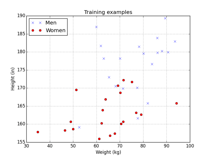
Classify a person as male or female based only on their height and weight.

As a training set, I’ve created a set of 40 individuals (i.e. 20 male, 20 female) based on the US census data. Since a person’s height and weight change as they get older, I simplified the problem a little by only using data from 19-year-old individuals. Each point on the graph is a person, represented by their height and weight, with the blue points being men and the red points being women.

By Jay Turcot, Lead Scientist, Affectiva 

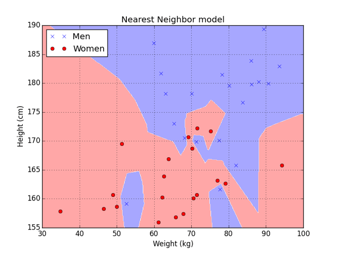
Lets start with Nearest Neighbor as it is quite straightforward. Nearest Neighbor is an algorithm which looks for the most similar training point and uses that point’s class as its answer. In other words, during the training phase, Nearest Neighbor takes all the training samples and saves them as well as the classes they belong to; our “model” is therefore all the training data. During the test phase, Nearest Neighbor takes a new datum and compares it with each point in the training data in order to find the closest match. It then reports back the class associated with the closest match.

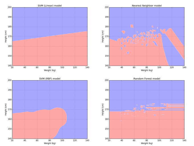
The resulting model can be displayed using a decision region graph. Here areas of the graph shaded blue are where the model would say a person is a male. Areas of the graph shaded red are where the model would say a person is a female.

This approach can be effective but suffers from drawbacks: there is no condensation or generalization of our training data in any way. If we use this approach with billions of training samples, the simple step of finding the ‘most similar example’ can take a VERY long time and would require more memory than a typical computer or mobile device has available.

As a student, Nearest Neighbor would be slow and meticulous almost to a fault. It does not try to extract any general trends or learn any patterns and as a result can make a lot of mistakes. Also, the more training examples we give our meticulous student Nearest Neighbor, the longer it will take to come up with an answer.

Let’s instead look at a simpler algorithm: a Linear SVM (Support Vector Machine). During training, the Linear SVM examines all the training data and finds a single line that “best” separates the men from the women, and remembers only the line. While the methodology for finding this line is relatively complex compared to the Nearest Neighbor, the resulting model, a line that separates men from women, is very simple and also very fast to compute. During testing, the Linear SVM calculates on which side of a single line a person falls–the side for men, or the side for women–and uses that as the answer.

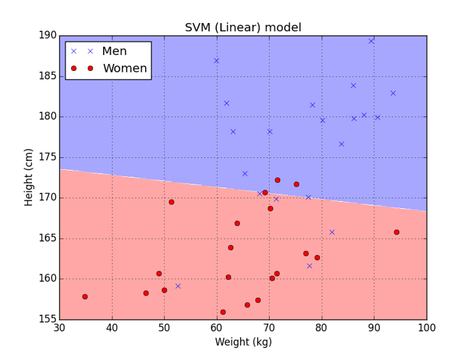
The approach of using a line, or linear separator, like the Linear SVM has some advantages. It is VERY fast and its speed doesn’t decrease no matter how much training data it is given. Linear SVMs also have their own drawbacks. If we were trying to solve a more complicated problem, a straight line might not be able to separate our two classes of people and a Linear SVM might not be accurate. Even with this simple problem, the model isn’t a perfect fit for the training data and some mistakes were made. This is due to the fact that height and weight alone are not enough to perfectly distinguish men from women.

As a student, the Linear SVM is quick to come up with an answer based on gut feel. It is very fast to give an answer and will be great for simple problems. However, on more complex problems, where there are often exceptions to the rule, its gut feel might lead it astray.

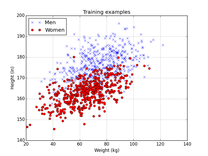
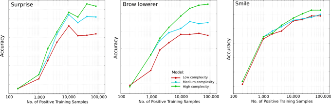
In between, there are a large number of algorithms which all have their own strengths and weaknesses. Some are faster than others, and some are better at performing complex classifications. While the best classification algorithm may vary from one application to another, there usually exists a tradeoff between how accurate the model is, how fast the model runs, and how much data is needed to train the model. Below we can see some decision regions learned by different machine learning models on the same problem, this time trained with 500 men and 500 women.

Sidenote: For classification, I personally prefer families of machine learning techniques that allow the research to directly specify how fast and complex the model is. This lets you explore the tradeoff between speed and accuracy in detail and pick the algorithm that works best. This can be achieved through several different machine learning techniques and several algorithmic mechanisms which I won’t go into in this blog post.

One of the tasks performed by the research team here at Affectiva is to constantly explore new machine learning techniques and new training methodologies to see what works best for facial expression classification. As our pool of available data increases, we can begin to use some of the latest machine learning algorithms which typically require millions of training samples, such as deep learning techniques. These algorithms can model very complex problems and therefore show a lot of promise when we have enough data to train them.

All in all, working with machine learning is an exciting and challenging problem that at times really does feel like teaching a classroom full of students. Sometimes students can surprise us and perform extremely well in adverse conditions. Other times, we have high hopes for a student who lets us down. Day by day, we are constantly introducing new students to the classroom, experimenting with different teaching methodologies and seeing which of our students excel. The strongest students are tested for speed, accuracy and robustness and the best of the best graduate into the real world and are integrated into our product.